Data Analysis Tips for Marketers: Easily Cleaning Qualitative Data

By Tom Swanson, Engagement Manager at Heinz Marketing

Jump straight to the formulas

Novice analysts are often surprised how much time spent working with data is actually cleaning it so that the analysis itself can be done smoothly.  While some of us are delighted by data cleaning, others can find it rather tedious.  Either way, a well formatted data-set makes analysis much easier and allows for you, the budding analyst, to quickly find the best insights and show your expertise.  Depending on the size of your data set, this can be a daunting task, but thankfully, there are many simple and flexible functions that make the process go much faster.

In this post we will be talking about cleaning qualitative data.  Qualitative data is great, it gives context to otherwise cold and numeric data sets.  However, that comes at a steep price of being hard to analyze at scale.  In many survey questions, the answers are non-numeric, but you want to see answer frequency, pivot the data, or be able to segment by answers.  Well, there are a few options for doing this, the right one depends on how your raw data is formatted.  Let’s dive in!

Answers are in the same cell, separated with commas

For the sake of simplicity, we will use a “Select all that apply” question.  This is not exactly qualitative data, but it works to demonstrate the functions, which can be applied in a variety of ways.  So, take a question like this:

Which animals would you want as pets? (select all that apply)

1. Crocodile
2. Cat
3. Bear
4. Spider

Your data may wind up looking something like this image:

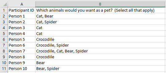
Google Sheets, for example, delineates “select all that apply” questions like this, with values separated by commas in the same cell.  We could count this manually, filter it, or use Google’s analysis interface, but large-scale segmentation will be tedious with data like this.

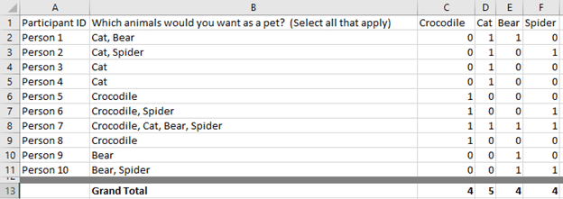
We want it to be easier to analyze, which would benefit from converting the text answers to simple 1’s and 0s.  Like this:

This would be easy to do manually for a small data set like these 10.  But what if you had 100?  5000?  Luckily, there is a formula that can help us with this.  It looks intimidating, but it is quite simple and I will break it down piece by piece.

=IF(ISNUMBER(SEARCH(value, target)), 1, 0)

Note: for Google Sheets, the formatting is almost identical and it still opens with an IF statement.  It uses a concept called a “regular expression” and seeks a match, but the output is the same.  I will go into this another time.  See the Google formula above for the different vocabulary and syntax.

The formula has 3 functions in it.  Working from the inside, out:

SEARCH

The SEARCH function is useful for numerous things, but what matters here is that it returns a number if a string appears in a cell.  If the value does not appear in the cell, you will get a #VALUE! error.  If you want to learn more about it, here is a short post.

ISNUMBER

The ISNUMBER will tell you if a value is a number or not.  If it is a number, it will say “True” and if not, “False”.

#VALUE! is not a number.  Hopefully you are starting to get a sense for how the rest of the formula works.

IF

Ahh the IF function, the building block of glorious Excel logic.  How it functions is pretty simple:

=IF(parameter, return value if True, return value if False).  Basically, if it looks like this =IF(parameter, A, B), you will get A if the parameter is met, otherwise you get B.

So back to our formula, hopefully you can make sense of it now.  Here it is again:

=IF(ISNUMBER(SEARCH(value, target)), 1, 0)

The function uses SEARCH to get a number if the target answer appears in a cell, then ISNUMBER converts that to True/False, and IF will return a 1 if ISNUMBER True was returned, and 0 if False.

For Column C in the above image, the formula for cell C2 looks like this:

=IF(ISNUMBER(SEARCH(C$1,$B2)),1,0).

Bonus Excel/Google Sheets tip: The $’s keep column/row values static, so you can click and drag the formula across the other columns and to the bottom of the data set, and it will auto-update all the necessary cells.

Answers are in different cells

Another common format is that data gets returned with as many columns as possible answers, but the answers are not in a specific column related to that specific answer. Rather, the machine just puts the first recognized value in the first column and goes form there.

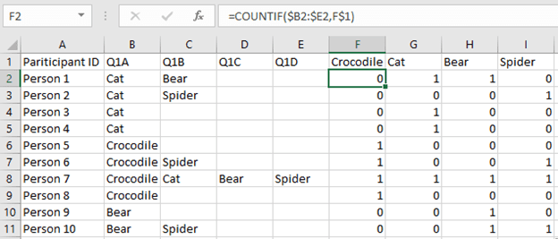
This is hard to imagine, so here is what it looks like:

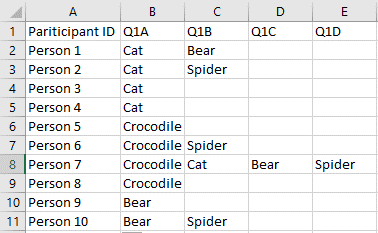
This is hard to analyze.  You cannot filter it, so you need to clean it.  Again for a 10 person data-set, it would be quickest to just do it manually, but as before, that falls apart at scale.  This is a simple fix.

Here is the function: =COUNTIF(range, value)

IMPORTANT NOTE: COUNTIF adds 1 for each instance of an answer that appears in a range.  Therefore, use this formula only if your values are unique to each participant and in their own cells.

In this case, our range for row 2 would be B2:E2.  We want to look for Cat in any of those cells.  So we make Cat a column and that becomes our value, then we put the formula in the next cell (F2):

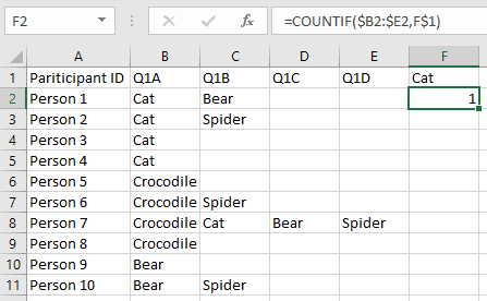
You can see the formula in the bar above.  Again the $s hold those column/row values constant so the formula can be dragged around.

Lovely, now we have a beautiful, clean data set that can show us how people answered our important question.

Now What?

These formulas are useful in more ways than just “Select All that Apply” questions!  They can be applied creatively to many different qualitative data sets.  You can use them to search for specific strings of text in larger qualitative responses, generate frequency maps and word clouds, segment responses by inclusion of these elements, and more.

As marketers, and analysts, it can be too easy to ignore qualitative data because it is hard to convert into metrics.  However, qualitative data includes huge amounts of context that can really improve your strategy game.  Having the tools to quickly and efficiently parse qualitative data will give you much more useful information, and allow you to sniff out the true story among all the words.

I am always on the look out for more formulas and ways to have fun with data, please reach out to me with any ideas or feedback!

Formulas:

To break out comma-separated strings in the same cell:
Excel: =IF(ISNUMBER(SEARCH(value, target)), 1, 0)
Google =IF(REGEXMATCH(target, value), 1, 0).
For isolated strings across a range of cells:
Excel & Google: =COUNTIF(range, value, 1, 0) – note that this will double count if values are not unique to each respondent.
If you want to know how these work and how to use them in a spreadsheet, I break them down with an example above.